Grammars and Parsers

MollyPages.org
"You were wrong case.
To live here is to live."

Home

Pages / Database / Forms / Servlet / Javadocs

/ License & Download / Tutorials / Cookbook

/ Contact & Hire

Parsing Topics

(Back to Molly Pages)
[Author: Hursh Jain]

For the best (by far) overall reference on this topic, see:

Parsing Techniques - A Practical Guide by Dick Grune and Ceriel J.H. Jacobs.

The section (below) on LL(1) recursive descent parsing is rather comprehensive and complete (I've worked out all the possible edge cases in the various examples).

Note 1: Keep in mind that a lot of theory-of-computation literature takes a pseudo-mathematical approach with "sets", which is the last refuge of the untalented and uninspired. A real mathematician would, in my opinion, -barf- at the mindless, un-intuitive and useless formalism-for-its-own-sake approach.

Note 2: The best approach, as always, is to both write and examine as much real code and real programs as possible.

Grammars

Grammars describe hierarchical structures.

These structures can be self-similar or nested at various levels.

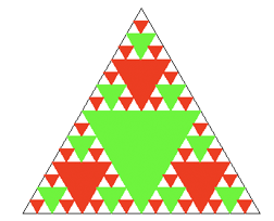
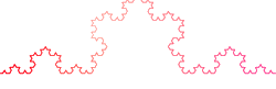
A self-similar structure is called a fractal. There are many ways to describe fractals.

One such way is Lindenmayer-systems (L-systems). These are a type of grammar that can generate/describe recursive structures like Koch curves, Sierpinski triangles and various other fractals.

Here's a simple Grammar:

X -> a X b

The structure X is composed of a X b ...which contains X itself ! Therefore this is self similar/fractal structure, because it contains itself.

Replacing X by its right hand side, we get:

  -> a (X -> a X b) b
  -> a a X b b

and so on:

  -> a a (X -> a X b) b b

until we get tired and stop using the X entirely (we say X -> ε [empty/erased])

One can think of a grammar as a recursive drawing template, where parts of the drawing (called non-terminals in grammar speak) are replaced with other drawings, possibly even with the same drawing as the parent drawing.

  -> a a a b b b

The left and right hand sides in a grammar rule are arbitrary.

Here's another grammar with 3 rules.

    X -> a X b
    X a Y -> c
    Y -> b X a Y

Using, say, the 3^rd rule from the above grammar, any or all of the following are possible and arbitrary.

```
 Y -> b X a Y
   -> b a X b a Y
```
```
 Y -> b X a Y
   -> b c
```
```
 Y -> b X a Y
   -> b b X a Y
```

...and so on. The application of all applicable rules at every possiblity gives us a collection of sentences (i.e., structures) generated by that grammar.

Structured Computer programs in most common high-level programming (HLL) languages can also be described via a grammar (although this is nearly not as much fun as a graphics L-system).

Consider a program which contains nested if...else statements. We can say:

X   -> if (condition) {
         X 
         } 
         else { 
         X 
         } 
    -> ε (epsilon, i.e., empty)

The X can be replaced by other if...else statements. For example:

X   -> if (condition) {
         X   -> if (condition) {
                  X -> ε (epsilon, i.e., empty)  
                  } 
                  else { 
                  X -> ε (epsilon, i.e., empty) 
                  } 
         } 
         else { 
         X -> ε (epsilon, i.e., empty) 
         }

..resulting in the program:

X   -> if (condition) {
            if (condition) {
            } 
            else { 
            } 
         } 
         else { 
         }

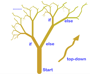
Computer programs are nested. Grammars describe nested structures.

So, to parse a computer program (like the if..else program above), we try to create a grammar that we think can be/was used to generate the program.

We use this grammar to try to generate all possible programs, including the program we are analyzing. The grammar can create an arbitrary number of different possible programs/structures, including programs we care about.

If we cannot generate our program from the grammar, then either (1) that particular grammar cannot be used for this program or (2) there is a syntax error in the program.

If the program we generate matches the program we have, we have a fit. (this is known as the top-down approach).

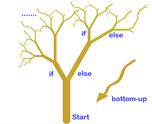
Alternately, can also start with the given program, and try to mash up the individual pieces into bigger boxes (higher up in the grammar). If all the pieces fit in the larger boxes, we end up with the original grammar (the largest box being the start rule of the grammar).

In either case, we note down the series of grammar rules/productions that were applied to get to the end result. We can then use these same rules to write another lower level program (say in machine code). We have effectively transformed one language into another.

Note, there might be more than one way to generate our program from the grammar (using the top-down approach) or more than one way to consolidate our program (using the bottom-up approach). This is perfectly fine but such grammars are called ambiguous. For keeping things simple and to give programs we write a definite and single meaning, we tend to disallow ambiguous grammars when describing programming languages.

While choosing grammar rules, we can also use the program we are analysing to help reduce the number of possible choices that we have to follow in our grammar. For example, if the next input sentence in our program is "then", and we have the following 2 rules:

X ->  if then X
X ->  if      X

We only need to choose the first rule (since the second rule doesn't contain then at this point).

Restricted grammars with (1) only one non-terminal on the left hand side and (2) the ability to choose a single top-down rule at any point (based on the program we are analysing) are called LL(1) grammars.

Consider this simple program:

if ( x = 1 ) 
    print  "hello" 
else
    print  "goodbye"

Corresponding to this is the simple grammar:

X    -> if ( COND ) STMT else STMT
COND -> letter == number 
STMT -> print text

Applying our grammar and noting the rules used, we get the parse tree:

RULE:
X ->
  if 
    COND -> 
      letter: x
      =
      number: 10
    STMT ->
      print 
          text: "hello" 
  else ->
    STMT ->
      print text: goodbye"

This parse tree is then converted into machine code that may look like:

1:   LOAD            X FROM MEMORY [100]
2:   COMPARE         X 1
3:   JMP_ON_EQUAL    GOTO LOCATION 10
4:   PRINT           "goodbye"
5:   STOP
10:  PRINT           "hello"
11:  STOP

Both the parsing of the program (in a parse tree) and the conversion of the parse tree into machine code can be automated and done by a computer program. Write a program to translate other programs...pretty cool!

Such a program is called a compiler/translator.

This leads to a chicken and egg problem. If our compiler/translator itself is a computer program written in a high level language, how do we use it ? We need to first convert the compiler program to machine code in order to run it. But we cannot convert the program to machine code because we don't have any compiler in machine code and we need the machine code version to compile any program at all (including itself).

Bootstrapping The solution is called bootstrapping. In its simplest form, it means we first use the human brain to convert the compiler-program written in our high level language into machine code. (or write the compiler-program in machine code directly). Once we have this initial program running, we can use it to compile any other high-level programs written in our programming language. These high level programs could include our original high level compiler-program or even other more sophisticated compiler-programs with more features and larger syntax.

It is not intuitively obvious whether such a compilation/translation is even achievable via computer/mechanical means. But it turns out that computers, indeed are capable of doing this conversion.

A little recap of grammars

Dealing with choices. There are two basic ways to deal with choices when parsing grammars.

1. Breadth first

Split at each decision point (try each option at every decision point in parallel)

2. Depth First

Keep track of each decision point and backtrack on failure.
Trying to fit Grammar rules

1. Top down

Choose rules from the grammar (starting from the start rule) and try to derive the entire text. The sequence of productions chosen is the parse tree.

2. Bottom up

Start from tokens from the text, try to reconstruct them into a production rule that could have derived those tokens and so on until the entire text is consumed. The sequence of productions again gives the parse tree.
Reading the text to parse.

1. Non-Directional

All of the source to be parsed is in memory and/or can be analyzed at the same time.

2. Directional

The text to be parsed is read piece by piece and all of it is not analyzed at the same time.

The following table shows how the above 3 dimensions interact.

	Top Down	Bottom Up
Directional	Unger method	CYK method
Non directional	Breadth-First Greibach method Depth-First backtrack These are typically implemented using recursive descent.	Breadth-First Earley method Depth-First backtrack These are typically implemented using shift/reduce.

Backtracking implementation note If implementing a backtracking parser in the general case, it is important to keep track of every decision point and backtrack back to each such point as needed. Consider:

S -> a X b
X -> c d
  -> c

Consider the input: a c b

Using the above grammar, we use:

S -> a X b
  [1]
  -> a X -> cd b
  -> a c d b   
  -> Match fails at d
  [2] backtrack.
  -> a X -> c b
  -> a c b
  -> Matches

Now consider the input: a c d b

S -> a X b  
  [1]
  -> a X -> c b
  -> a and c both match.
  -> Match fails at 'b' ('d' in the input)
  [2]
  -> We need to backtrack and try another option. Even though the production 
  choice X -> c matched, it caused a failure later on, so we backtrack past
  this successful choice (since we keep track of all choices) and try another 
  production.
  -> a X -> cd b
  -> This matches the input.

Regular Grammars

Regular grammars generate flat sentences with no nesting/hierarchy. Note, that is a general case, any given or particular heretical structure with a a-priori known level of nesting can be generated by a regular grammar.

Regular grammars have production rules of the form:

S -> any combination of Terminals. There can only be 1 non-terminals that
     can only appear left most or right most.

There can be more than one production for a given left hand non-terminal and ε productions are allowed.

S -> X      
  -> Y
  -> ε

For example:

X -> a X
X -> a b X | ab

Repetitions are specified as:

X  -> a    | ε        0 or 1 a    a?
X  -> a X  | ε        0 or n a's  a*

X  -> a X'            1 or n a's  a+
X' -> a X' | ε

Back-references are not regular. For example to match: beri beri, one might say:

(.*)\1

However, this is not a regular expression but a context free grammar of the kind:

X  -> YY 
Y  -> anychar Y

Implementation Note Some implementations of regular expression matchers use NFA's. These are equivalent to a depth first backtracking search and can involve exponential time for expressions like (.*) or (.*)* especially if no match is found (or all matches need to be found). This does not occur for DFA's or breadth first searchers.

A very common task is to find a delimited string with embedded escape sequences. The delimiters can be any character or string, for example:

Delimited by a quote: ".....foo\n \"....."
Delimited by <x>:    <x>.....\<x>.....<x>

Regular expressions/grammars can be used to match these constructs. For example: ".....foo\n \"....." is matched by "[^"]*"

<x>.....\<x>.....<x> is matched by "(\.|[\"])*". This regex is slightly tricky since, we cannot use character classes for more than one character. We cannot say: "[^<\x>]*" since that would match any of < \ x > singly (not as a sequence). The \. matches the escape sequence of ANY length such as \<xmp> or \" first. Then the second alternative [^\"] matches any char which is not a \ or a "

A lexer is a program that breaks down its input into tokens. The tokens are usually specified by regular grammars/regular expressions.

Implementation Note The following functions are typically found in lexers:

Name	Description
peek() peek(buffer)	Returns the next character in the stream without consuming it.
unread()	Push-back the character back into the stream. - Useful when reading characters in a loop until a specific character (say whitespace) is encountered. There is 1 extra read to break out of the loop and we have to put that extra character back into the stream. - Note: peek() gives equivalent functionality. However, using peek(), the loop is structured in a different way: keep peeking() until the next character is not what we are looking for.
read()	reads and returns a character from the input. Keeps track of line and column per every read and suitably increment line, col as needed. There are 2 usual ways to return a EOF value: throw an Exception return a special value (like -1) which is guaranteed to not occur in the input itself.
skipPast(character) skipPastXXX() skipUntilXXX() For example: skipPastWhitespace() or skipPast(' ')	Keep reading until XXX is skipped or is reached. Use peek() or unread() as needed.
expect(character/string)	Convenience method to expect a character/string in the input and throw an error if not present.

Regular grammars can also be visualized as finite automata. Switching from state to state is the same as following a particular production in the grammar. An automaton switches states based on the next input item that it reads. A non deterministic finite automa (NFA) is the same as a grammar in which more than one production/rule can be chosen at a given point. One can then choose several productions which is the same as being in more than one state at a given time.

An implementation may accomplish this in parallel or via backtracking or via converting a NFA to a DFA (which is essentially in parallel)

Finite automatons are often easier to visualize than the equivalent grammar notation.

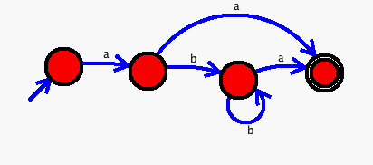
Here's a grammar that generates sentences of the form: ab*a

S -> a X a
X -> b X
  -> ε

Equivalent finite automaton:

Context Free Grammars

Context free grammars have production rules of the form:

Only 1 Non Terminal -> any combination of Terminals and Non-Terminals.

Like regular grammars, context free grammars can also have more than one production for a given left hand non-terminal.

A -> X      
  -> Y

For example:

A -> X y Z   
A -> X y X

Since the same non-terminal can occur on both sides of a terminal symbol (like X y X), arbitrarily deep nesting on the left side has to be matched by the equal symbol on the right side. Therefore, nesting to any depth can be represented by context free grammars.

This is equivalent to just keeping a count of the depth on the left side and matching that with the right side, so we are simulating a simple counter variable (or equivalently a stack) with this grammar.

Now we get into the practical mundane aspects of grammars.

Grammars can often be simplified by the following methods.

Eliminating ε-productions

Example 1

S  -> aA
A  -> b
   -> ε  [to be eliminated]

A derives ε. Look for all other productions in which

appears on the r.h.s. An ε on the r.h.s means that the production can disappear (i.e., A*) and removing ε converts a choice between a production vs. ε to a choice between other productions. For example:

S  -> a A

Add another production with A removed. (i.e, apply A -> ε).

1) Add:
    S  -> a
2) Then remove the ε-production:
    A  -> ε

Final result:

S  -> a A
   -> a    [added]
   -> ε  [removed]
A  -> b

Note:

We have to remove A in all possible combinations (first, second, both etc) since these removals derive different sentences. If we have

1   S -> A B A
2   A -> x
3   A -> ε

Then we cannot just replace:

1   S  -> x B x

Instead we have to add the following:

1      ->  B A
2      ->  A B
3      ->  B

and then apply: A -> ε in all of the above. This results in:

2   S  ->  B x
3   S  ->  x B
4   S  ->  B

Now remove: A -> ε, so we get:

1   S  -> A B A
2   S  ->   B A
3   S  -> A B
4   S  ->   B
2   A  -> x

Example 2

This is a good example.

1     S  -> A B A C
2     A  -> a A   
3        -> ε
4        -> b B
5        -> ε  
6        -> c

Replacing A -> ε, we now get additional productions:

1     S  -> ABAC 
1.1      ->  BAC  [first A removed]
1.2      -> AB C  [second A removed]
1.3      ->  B C  [both first and second A removed]

2     A  -> aA     
2.1   A  -> a     [A removed]

Replacing B -> ε in all of the above, we get the following additional rules. this now becomes:

1     S  -> ABAC  
1.4      -> A AC   (remove B from 1 above)
1.5      ->   AC   (remove B from rule 1.1 above)
1.6      -> A  C   (remove B from rule 1.2 above)
1.7      ->    C   (remove B from rule 1.3 above)
       
4     B  -> bB     
4.1   B  -> b      (remove B)

Note, two of the resultant rules are of the form


S -> AC

which can be consolidated. These extra rules are added to the original grammar and the ε-rules are removed. The final result:

S  -> ABAC
   -> ABC
   -> BAC
   -> BC
   -> AAC
   -> AC
   -> C 
A  -> aA
A  -> a
B  -> bB
B  -> b
C  -> c

Eliminating Unit Productions

1   A -> B
2   B -> xy

In this grammar, A -> B is called a unit production. A unit production is a rule in which the right hand side of the rule contains only one symbol and that symbol is non-terminal. In this example, only B appears on the r.h.s of rule 1 and therefore this is a unit rule.

This rule does not add anything to the kind of sentences produced. The above grammar can be written more simply as:

A -> x y

Eliminating unit productions makes grammars clearer. To eliminate unit productions:

1) Select a unit production from a pair of grammar rules that look like:

A -> B
B -> ∂   [∂ is any non-unit right hand side]

Add:    A -> ∂
Remove: A -> B

3) Resulting grammar:

A -> ∂

Example 1

A -> B
B -> C
C -> D
D -> x

Start with:

A -> B

Select:

B -> C

This is a unit production too, so select

C -> D

This is a unit production too, so select

D -> x

This is a non-unit production, so use:

A -> x

The final grammar is:

A -> x

Example 2

1   S -> AB
2   A -> a
3   B -> C
4     -> b
5   C -> D
6   D -> E
7   E -> a

Three unit productions exist

3   B -> C
5   C -> D
6   D -> E

Goal: eliminate B -> C. No non-unit C -> ... productions exist. Stop. Try Step (2).
Goal: eliminate C -> D. No non-unit D -> ... productions exist. Stop. Try Step (3)
Goal: eliminate D -> E. Aha. E -> a is a non-unit rule. So:

Add the non-unit rule:
  D -> a  (because E -> a)
Remove the unit rule:
  D -> E

Start again. The following are still left to eliminate.

B -> C
C -> D

Following the steps as before, we get: For rule C -> D

Add: 
  C -> a
Remove:
  C -> D

and then for Rule B -> C

Add: 
  B -> a
Remove: 
  B -> C

The grammar now looks like:

1   S -> AB
2   A -> a
3   B -> a
4     -> b
5   C -> a
6   D -> a
7   E -> a

However, since C, D and E are unreachable from S, the final grammar is:

1   S -> AB
2   A -> a
3   B -> a
4     -> b

Eliminating Left Recursion

This is useful for top down parsing (in order to be able to break out of a loop while deciding which production to choose). Consider the grammar:

A -> A x 
  -> y 
  -> ε

Applying the rule A -> ε initially, we get ε. Applying the rule A -> A x we get:

Ax
Axx
Axxx

and then we get:

Ax    -> x      (A -> ε)
Axx   -> yxx    (A -> y)
Axxx  -> yxxx   (A -> y)

Therefore the grammar gives us either an ε, or [0_or_1 y followed by 0_to_n x]. Therefore, eliminating left recursion we get:

A  -> y A' | ε  (1 or 0 y)
A' -> x A' | ε  (0 to n x's)

Similarly, the following grammar (different than the one above because it contains no epsilon):

A -> A x             
  -> y

becomes:

A  -> y A'      (1 y)
A' -> x A' | ε  (x's)

The following grammar

A -> A d  | A e | a B | a C

becomes:

A  -> a B A' | a C A'
A' ->   d A' | e A'  | ε

Deterministic parsing of context free grammars

Parsing context free grammars is easiest using a top down, breadth-first searching, wherein the source text determines the rules that can be applied (starting from the start rule) and if more than one rule can be applied, than each choice is examined in parallel. This is called non-deterministic parsing.

This however can have a large time/memory use and in practice, therefore to cut down on having to chooose all possible rules, most parsers are deterministic. This means that the grammar rules are structured in such a way that depending on the next few source tokens [typically, 1 hence LL(1)], only 1 grammar production can be applied. (hence the rules can be applied deterministically).

First Sets are defined as follows:

For some production:

S -> α Y β       [where α, Y, β could be terminals or non-terminals]

first(S) = first(α Y β) 

If α is a terminal
    first(α Y β) = α
else
    calculate first(α)
 
if first(α) contains ε (can contain others too)
        first(α Y β) = first(α) - {ε} U first(Y β)   [Note 1]
else  // (if first(α) does not contain ε)
        first(α Y β) = first(α)

Note 1: first(Y β) is recursively calculated in a similar manner. However
if we get to first (β) and that does contain ε, then since β was the last
non-terminal, that final ε is included in the first set. (we must
look at follow sets in this case to decide whether to choose ε).

For a grammar to be LL(1), first sets for all productions (right hand sides) for any ONE left hand side must be disjoint.

An Example

S   -> A C B
    -> C b B
    -> B a
A   -> d a
    -> B C
B   -> g | ε
C   -> h | ε

first (S -> ACB) = first (A C B)  
                = first (A)
                = {d, g, h, ε}
                first (A) contains ε
                = {d, g, h, ε} - ε + first (C)
                = {d, g, h} + {h, ε}
                first (C) contains ε
                = {d, g, h} + {h, ε} - ε + first (B)
                = {d, g, h} + {h, ε} - ε + {g, ε}
                first (b) contains ε. But we do not subtract
                ε since B is the last item in our  S -> A C B
                = {d, g, h, ε}
            
first (S -> CbB) = first(CbB)
                = first(C)
                = {h, ε}
                = {h, ε} - ε + first(b)
                = {h, b}

first (S -> Ba) = first(Ba)
                = first(B)
                = {g, ε} - ε + first(a)
                = {g, a}
                
first (S)       = first(ACB) = {d, g, h, ε}
                + first(CbB) = {h, b}
                + first(Ba)  = {g, a}

Since the above 3 sets (for the same left hand rule S) are not disjoint, this grammar is not LL(1).

Let's go ahead and find first sets for other productions in this
grammar anyway.

first (A -> da) = first(da) 
                = d 
first (A -> BC) = first(BC) 
                = first(B)
                = {g, ε}   //we know first B already from above, time-saver!
                Since first(B) contains ε
                = {g, ε} - ε + first(C)
                = {g} + {h, ε}
                Since C was the last item in the rule, we do not subtract ε.
                = {g, h, ε}

first(B -> g ε) = first(g, ε)
                = {g, ε}
                The last ε is included

first(C -> h ε) = first(h, ε)
                = {h, ε}
                The last ε is included

If ε exists in the grammar, then how do we know when to choose the ε-production in a deterministic parser ? (we could potentially choose ε for that production every time). For example, if:

A   -> aB | ε
B   -> a

then we could potentially choose A -> ε (since both {ε, a} are in A's first set.

A -> ε is the right choice in a deterministic parser, when the next input terminal matches the symbol immediately following A in some production. The set of all terminals following A are known as A's Follow Set.

A   -> a | ε
X   -> A b

b follows A in the production X -> A b.

Therefore: follow (A) = b and we can use the following production selection table.

STATE Next symbol

b a

A A -> ε A -> a

Generally speaking, to calculate follow sets:

1. For a rule of type:
A -> α X β       
     where α, β are any sequence of terminals & non-terminals

follow (X) = first (β) if first(β) does not contain ε
             else //if first(B) contains ε
             = first(β) - ε U follow(A)  [note 1]

        
Note 1. This is because if β contains ε, then whatever follows A will follow β (since
all of β can become an empty string).

2. Rules of type:
    X -> a
    X -> abc
    X -> ε
do not add anything to the follow set of X itself.

3. For a rule of type:
A -> α X       (X is the last item in the rule)

follow (X) = follow (A)    [note 2]   
Note 2. Because whatever follows X in some rule will also follow A.

Note: ε is never in a follow set. (but EOF (end of
file) may be). The entire point of follow sets is to figure out when to choose
A -> ε for the current non-terminal A (follow sets are useful only
for non-terminals whose right hand side can go to ε). If ε is also in the follow set,
then that would mean the current non-terminal should always go to ε.

Therefore, in the presence of ε, the general rule for deterministic LL(1) parsing is:

A -> α
A -> β

1. First sets for a given left hand non-terminal must be disjoint. For example,
first (A -> α), first (A -> β) must be disjoint.

2. Furthermore, all first (A) sets AND all follow (A) sets must be disjoint. If
the first and follow sets were not disjoint, then we would not know whether for a given
non-terminal we should apply a non-ε rule or choose ε for that non-terminal.

3. If first (α) does contain ε, then as per rule 1, all other first sets of A
must be disjoint from (A -> α) and therefore no other first set for A can contain ε.
That is:

    Follow (α) ∩ First (β) = ∅

Some more examples of calculating first/follow sets.

Example 1

[Show/Hide answer]

S   -> a A b
A   -> c d
    -> e f

This grammar contains no ε-rules, so there is no need to create follow sets.

first (S -> a A b)  = a
first (A -> c d)    = c
first (A -> e f)    = e

The production choice table is:

STATE	Next symbol
	a	b	c	d	e	f	$ (end of input)
S	S->aAb
A		A->cd		A->ef

Example 2

[Show/Hide answer]

X   -> A B b c | d e
A   -> a | ε
    -> b | ε

first (A)   = {a, ε}
first (B)   = {b, ε}
first (X -> A B b c) 
            = first(A)
            = {a, ε} - ε + first(B)
            = {a} + {b, ε} - ε + first(b)
            = {a, b}
first (X -> d e) 
            = {d}

follow (A)  = first(B b c)  [since B follows A in rule X -> A B b c]
            = first(B)
            = {b, ε}
            Since first(B) contains ε
            = {b, ε} - ε + first(bc)
            = {b}
follow (B)  = {b}       [from rule: X -> A B b c]

follow (X)  = $ (e.o.f)

This is a interesting grammar. The first sets for X are disjoint from each other and likewise for A and B. However:

first (B) is not disjoint from follow (B)

first (B) = {b, ε}
follow(B) = {b}

As per the general deterministic rules, this means the grammar is still not deterministic. The production choice table is:

STATE	Next symbol
	a	b	c	....
X	X->ABbc	X->ABbc
A	A->a	A->ε
B		B->b B->ε

The following inputs are valid for this grammar:

abc
abbc

However, abbc neither can be parsed deterministically, since if we deterministically:
- always choose B->ε in the table above, then we can never parse abbc and
- always choose B->b, then we can never parse abc.

Of course, both sentences can be easily parsed using say a top-down breadth-first non-deterministic parser.

Example 3

[Show/Hide answer]

A slightly modified version of Example 2.

X   -> A b c 
A   -> a | ε

first  (X)  = first(A)
            = {a, ε} - ε + first(B)
            = {a} + {b, ε} - ε + first(b)
            = {a, b}

first  (A)  = {a, ε}
follow (A)  = {b}       [from rule: X -> A b c]

The production choice table is:

STATE	Next symbol
	a	b	....
X	X->Abc	X->Abc
A	A->a	A->ε

Example 4

[Show/Hide answer]

S   -> A a A b
    -> B b B a
A   -> ε
B   -> ε

first (S->AaAb) = first(AaAb) 
                = first(A) 
                = {ε} - ε + first(aAb)
                = {a}
first (S->BbBa) = first(BbBa) 
                = first(A) 
                = {ε} - ε + first(bBa)
                = {b}
                
Since ε-productions exist, we will calculate follow sets.
                
follow (S)      = $ (eof)

follow (A)      = first(aAb)  [from S->AaAb, A-->aAb]
                    +
                  first(b)    [from S->AaAb, AaA-->b]
                = {a, b}

follow (B)      = first(bBA)  [from S->BbBa, B-->bBa]
                    +
                  first(a)    [from S->AaAb, BbB-->a]
                = {b, a}

The production choice table is:

STATE	Next symbol
	a	b
S	S->AaAb	S->BbBa
A	A->ε	A->ε
B	B->ε	B->ε

Example 5

[Show/Hide answer]

S'  -> S$       [$ is eof]
S   -> q A B C
A   -> a | bbD
B   -> a | ε
C   -> b | ε
D   -> c | ε

first(S')       = first(S)      = {q}
first(S)        = first(qABC)   = {q}

first(A->a)     = first(a)      = {a}                   
first(A->bbD)   = first(bbD)    = {b}

first(B->a)     = first(a)      = {a}   
first(B->ε)     = first(ε)      = {ε}

first(C->b)     = first(b)      = {b}   
first(C->ε)     = first(ε)      = {ε}

first(D->c)     = first(c)      = {c}   
first(D->ε)     = first(ε)      = {ε}

Since ε-productions exist, calculate follow sets.

follow(S')      = first($)      = {$}
follow(S)       = first($)      = {$}
follow(A)       = first(BC)     [from qA->BC]
                = first(B)
                 = {a, ε} - ε + first(C)
                = {a}        + {b, ε}
                Since first(C) contains ε and C is the last non-terminal
                on the right hand side of this rule:
                = {a} + {b, ε} - ε + follow(S)
                = {a, b, $}
follow(B)       = first(C) 
                = {b, ε} - ε + follow(S)
                = {b, $}
follow(C)       = follow(S)
                = {$}
follow(D)       = D is the last non-terminal A->bbD, therefore
                = follow(A)
                = {a, b, $}

The production choice table is:

STATE	Next symbol
	q	a	b	c	$
S'	->S$
S	->qABC
A		->a	->bbD
B		->a	->ε		->ε
C			->b		->ε
D		->ε	->ε	->c	->ε

Example 6

[Show/Hide answer]

S -> A
A -> aB
  -> Ad

first (A->Ad) = first(A) = .....

This is left-recursive and first cannot be computed for this grammar.

Example 7

[Show/Hide answer]

S -> aBDh
B -> cC
C -> bC | ε
D -> EF
E -> g | ε
F -> f | ε

first  (S)      = {a}
first  (B)      = {c}

first  (C->bC)  = {b}
first  (C->ε)   = {ε}

first  (D->EF)  = first (EF)
                = first(E) - ε + first(F)
                = {g, ε) - ε + {f, ε}
                = {g, f, ε}
first  (E->g)   = {g}
first  (E->ε)   = {ε}

first  (F->f)   = {f}
first  (F->ε}   = {ε}

The follow sets are:
follow  (S)  = $ (eof)
follow  (B)  = first(Dh)    [from the rule S->aBDh]
             = first(D)
             = {g, f, ε}
             Since this contains ε
             = {g, f, ε} - ε + first(h)
             = {g, f, h}
follow  (C)  = From rule [B->cC], C is last non-terminal and since C->ε 
             = follow(B)
             = {g, f, h}
follow  (D)  = {h}          [from the rule S->aBDh]
follow  (E)  = first(F)     [from the rule D->EF]
             = {f, ε}
             Since F was the last non-terminal in D->EF and first(F) contains ε
             = {f, ε} - ε + follow(D)
             = {f, h}
follow  (F)  = Since F->ε
             = follow(D)    [from the rule D->EF]
             = {h}

Note, in the above grammar, even though there is no direct production D -> ε even though ε is in D's first set. We always apply D->EF when we encounter any terminal in D's first set {g, f, ε}. When do we choose

D ->
ε

? When we encounter something in D's follow set which is: {h}. In that case, we still apply D->EF, and then E->ε and F->ε (since {h} will also be in both E and F's follow sets).

The production choice table is:

STATE	Next symbol
	a	b	c	d	e	f	g	h
S	->aBDh
B			->cC
C		->bC				->ε	->ε	->ε
D						->EF	->EF	->EF
E						->ε	->g	->ε
F						->f		->ε

Example 8

[Show/Hide answer]

A -> B C
B -> A x | x | ε
C -> y C | y | ε

first (A)       = first(B)
                = {first(A), x, ε}
                = first(A) leads to self-recursion, we are trying to
                find first(A) in the first place, but first(A) = first(B)
                and first(B) = first(A). This recursive term is ignored.
                = {first(A), x, ε}
                = since first(B) contains ε
                = {x, ε}- ε +  first(C)
                = {x} + {y, ε}
                = {x, y, ε}

first (B->Ax)   = first(A)
                = {x, y, ε} - ε + {x}
                = {x, y}
first (B->x)    = {x}
first (B->ε)    = {ε}

first (C->yC)   = {y}
first (C->y)    = {y}
first (C->ε)    = {ε}

follow (A)      = {x}               [from rule: B->Ax]      
follow (B)      = first(C)          [from rule: A->BC]
                = {y, ε}
                = {y} + follow(A)   [since first(C) contains ε and C is
                                    the last rule in A->BC]
                = {y} + {x}
                = {x, y}
follow (C)      = follow(A)         [from rule A->BC, since first(C) contains ε]
                = {x}

The production choice table is:

STATE	Next symbol
	x	y
A	->B C	->B C
B	->ε ->Ax ->x	->ε
C	->ε	->yC ->y

This grammar is not LL(1).

Well, that's it for parsing theory. If you made it this far, congratulations!

And here's a real world surprise - this page you are reading is itself compiled, using the same theory as above. We wrote a translater that takes server side tags (like jsp, asp, etc) but in our own syntax that we like.

Then we parse this page, create a syntax tree and output that into a chunk of Java code (a servlet).

Once we have a syntax tree (also called intermediate representation), we can output into many different end forms (via what is called a backend generator). Many times it is assembler code, or byte code. In this case, it is Java code!

Here's the grammar for Molly server pages.

And here is the actual parser (click on the class name to see the code).